⌛️ Approximate time to complete: 25 min.
In this tutorial you will learn how to orchestrate multiple decision models together with the Nextmv Platform from scratch, using Nextpipe.
💡 From now on, running multiple decision models is going to be known as a decision workflow.
Complete this tutorial if you:
- Are interested in orchestrating decision workflows with the Nextmv Platform and Nextpipe.
- Are fluent using Python 🐍.
To complete this tutorial, we will use an external example, working under the principle that it is not a Nextmv-created decision workflow. You can, and should, use your own decision workflow, or follow along with the example provided:
At a high level, this tutorial will go through the following steps using the example:
- Nextmv-ify the decision workflow.
- Run it locally.
- Push the workflow to Nextmv Cloud.
- Run the workflow remotely.
Let’s dive right in 🤿.
1. Prepare the executable code
If you are working with your own decision workflow and already know that it executes, feel free to skip this step.
The decision workflow is composed of one, or more, executables that solve decision problems. Decision workflows are typically lightweight, meaning that they are focused on the orchestration of decision models, and not on the models themselves.
The original example is a Jupyter notebook that can be broken down into two distinct parts:
A statistical model that predicts avocado demand based on price and other features.
An optimization model that determines the optimal price and supply of avocados based on the predicted demand.
For simplicity, we copied the cells of the notebook into a single script. Copy the desired example code to a script named main.py.
2. Install requirements
If you are working with your own decision workflow and already have all requirements ready for it, feel free to skip this step.
Make sure you have the appropriate requirements installed for your workflow. If you don’t have one already, create a requirements.txt file in the root of your project with the Python package requirements needed.
Install the requirements by running the following command:
3. Run the executable code
If you are working with your own decision workflow and already know that it executes, feel free to skip this step.
Make sure your decision model works by running the executable code.
Note that this code in particular produces interactive plots.
4. Nextmv-ify the decision workflow
We are going to turn the executable decision workflow into multiple Nextmv applications.
So, what is a Nextmv application? A Nextmv application is an entity that contains a decision model as executable code. An application can make a run by taking an input, executing the decision model, and producing an output. An application is defined by its code, and a configuration file named app.yaml, known as the "app manifest".
Think of the app as a shell, or workspace, that contains your decision model code, and provides the necessary structure to run it.
A run on a Nextmv application follows this convention:
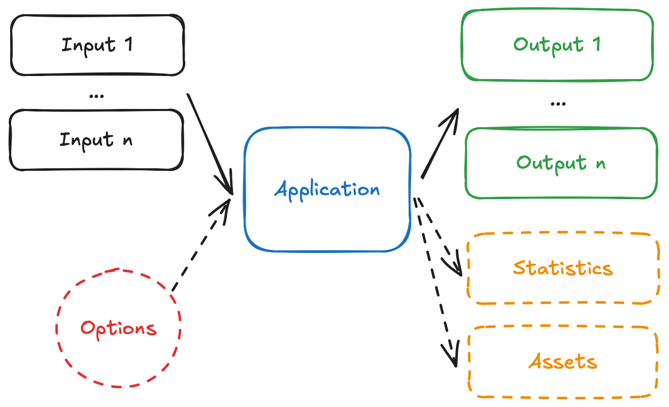
- The app receives one, or more, inputs (problem data), through
stdinor files. - The app run can be configured through options, that are received as CLI arguments.
- The app processes the inputs, and executes the decision model.
- The app produces one, or more, outputs (solutions), and prints to
stdoutor files. - The app optionally produces statistics (metrics) and assets (can be visual, like charts).
We are going to turn the Gurobi example into three distinct Nextmv applications:
- A
regressionapplication that will predict demand based on historical data. This application will output the regression coefficients. - A
decisionapplication that will receive the regression coefficients, alongside more input data, and will solve the optimization model to decide on pricing and avocado allocation. - A
workflowapplication that will orchestrate the previous two applications, running them in sequence to produce a final solution.
Each of the applications will follow Nextmv conventions. The following diagram shows the general idea of the three applications interacting:
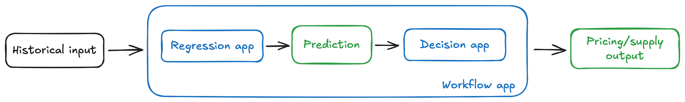
- The
workflowapp receives the initial input data. - The
workflowapp runs theregressionapp, passing it the historical data. - The
regressionapp produces the regression coefficients as output. - The
workflowapp then runs thedecisionapp, passing it the regression coefficients, alongside other input data. - The
decisionapp produces the final solution as output, and is returned by theworkflowapp.
Use workflows for orchestrating decision steps, not for implementing the decision logic itself.
As it was mentioned, decision workflows should be lightweight and focused on orchestrating steps that implement compute-intensive decision logic. In this case, the regression and decision steps are separate, independent applications focused on their respective tasks. The workflow application is only responsible for orchestrating the two steps. A bad practice would be to implement all business logic into the workflow application.
A key advantage of using Nextmv is that you can delegate the compute-heavy logic to individual applications, and you can use infrastructure to parallelize, distribute, and scale the execution of these applications as needed.
4.1. The regression application
Create a new directory named regression, and cd into it. Start by adding the app.yaml file, which is known as the app manifest, to the root of the directory. This file contains the configuration of the app.
This tutorial is not meant to discuss the app manifest in-depth, for that you can go to the manifest docs. However, these are the main attributes shown in the manifest:
type: It is apythonapplication.runtime: This application uses the standardpython:3.11runtime. It is a bad practice to use other specialized runtimes (likegamspy:latest); decision workflows should be focused on orchestration, and not on implementing decision logic.files: contains files that make up the executable code of the app. In this case only a singlemain.pyfile is needed. Make sure to include all files and dirs that are needed for your decision model.python.pip-requirements: specifies the file with the Python packages that need to be installed for the application.configuration.content: This application will usemulti-file, so additional configurations are needed. As you complete this tutorial, the difference between this format, andjsonwill become clearer.configuration.options: for this example, we are adding options to the application, which allow you to configure runs, with parameters such as the training size and random seed.
For this example, a dependency for nextmv (the Nextmv Python SDK) is also added. This dependency is optional, and SDK modeling constructs are not needed to run a Nextmv Application. However, using the SDK modeling features makes it easier to work with Nextmv apps, as a lot of convenient functionality is already baked in, like:
- Reading and interpreting the manifest.
- Easily reading and writing files based on the content format.
- Parsing and using options from the command line, or environment variables.
- Structuring inputs and outputs.
Because we are only working with the regression, we have reduced dependencies. These are the requirements.txt for the regression app.
Now, you can add the main.py script with the Nextmv-ified regression.
This is a short summary of the changes introduced for this application:
- Load the app manifest from the
app.yamlfile. - Extract options (configurations) from the manifest.
- The input data is no longer fetched from the Python file itself. We are representing the problem with several files under the
inputsdirectory. Ininputs/avocado.csvwe are going to write the complete dataset of sold avocados. Ininputs/input.jsonwe are going to write general information needed for the model, like the regions, peak months, and the initial year. When working with more than one file, themulti-filecontent format is ideal. We use the Python SDK to load the input data from the various files. - Modify the definition of variables to use data from the loaded inputs.
- Store the solution to the problem, and solver metrics (statistics), in an output.
- Write the output to several files, under the
outputsdirectory, given that we are working with themulti-filecontent format.
After you are done Nextmv-ifying, your Nextmv app should have the following structure, for the example provided.
4.2. The decision application
Create a new directory named decision, and cd into it. Start by adding the app.yaml file (app manifest) to the root of the directory.
The attributes shown in the manifest are largely the same as the ones exposed in the regression app. For simplicity, this app does not contain options (configurations).
For this example, the same nextmv dependency is introduced. Similarly to the regression app, we have reduced dependencies. These are the requirements.txt for the decision app.
Now, you can add the main.py script with the Nextmv-ified decision model.
This is a short summary of the changes introduced for this application:
- Load the app manifest from the
app.yamlfile. - Extract options (configurations) from the manifest.
- The input data is represented by several files under the
inputsdirectory. Ininputs/avocado.csvwe are going to have the same dataset of sold avocados. Ininputs/input.jsonwe are going to write the same general information needed for the model, plus information specific to the decision problem. Again, when working with more than one file, themulti-filecontent format is ideal. We use the Python SDK to load the input data from the various files. - Modify the definition of variables to use data from the loaded inputs.
- Store the solution to the problem, and solver metrics (statistics), in an output.
- Write the output to several files, under the
outputsdirectory, given that we are working with themulti-filecontent format.
After you are done Nextmv-ifying, your Nextmv app should have the following structure, for the example provided.
4.3. The workflow application
Create a new directory named workflow, and cd into it. Start by adding the app.yaml file (app manifest) to the root of the directory.
This application is a bit different than the others. It uses the json content format. This means that the application should receive json data via stdin and write valid json data to stdout. For simplicity, this app does not contain options (configurations).
This application orchestrates the regression and decision applications. To achieve this, we will use nextpipe, a lightweight library for handling decision workflows. We are also going to use nextmv for the convenience in handling I/O operations.
These are the requirements.txt for the workflow app.
Now, you can add the main.py script with the decision workflow.
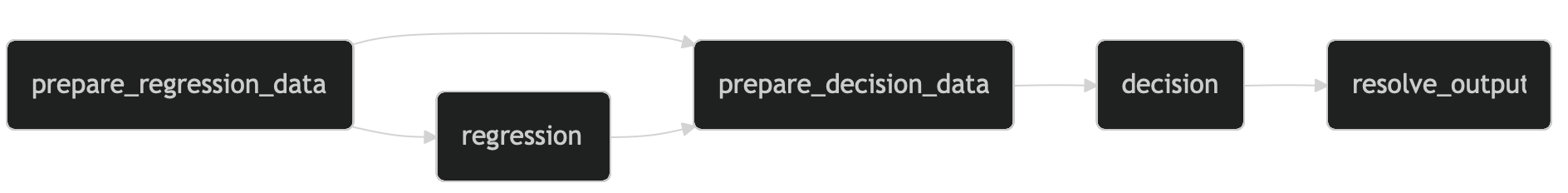
This is a short summary of what the application does:
- Read the input data from
stdin. - Set up the decision workflow.
- In the original example, the data was fetched from 2 URLs. The
prepare_regression_datastep downloads the data, merges it, and writes it to aworkflow_inputsdirectory. The resulting file, namedavocado.csv, is used by the subsequent steps, given that this input file is needed by both theregressionanddecisionapps. - The
regressionstep runs theregressionapplication, using the data from theworkflow_inputsdirectory. - The
prepare_decision_datastep prepares the inputs for thedecisionapplication. The results from theregressionstep (the regression coefficients) are copied to adecision_inputsdirectory, alongside the other input data. - The
decisionstep runs thedecisionapplication, using the data from thedecision_inputsdirectory. - The
resolve_outputstep collects the results from thedecisionstep, and writes them to anoutputsdirectory. It consolidates the solution and statistics into a single output dictionary.
- In the original example, the data was fetched from 2 URLs. The
- Write the output of the decision workflow to
stdout.
To run the workflow, here is the input data that you need to place in an input.json file.
After you are done setting up the workflow application, it should have the following structure.
Now you are ready to run the decision workflow 🥳.
5. Create an account
The full suite of benefits starts with a Nextmv Cloud account.
- Visit the Nextmv Console to sign up for an account at https://cloud.nextmv.io.
- Verify your account.
- You’ll receive an email asking to verify your account.
- Follow the link in that email to sign in.
- Log in to your account. The Nextmv Console is ready to use!
Once you have logged in to your account, you need to fetch your API key. You can do so from your settings.
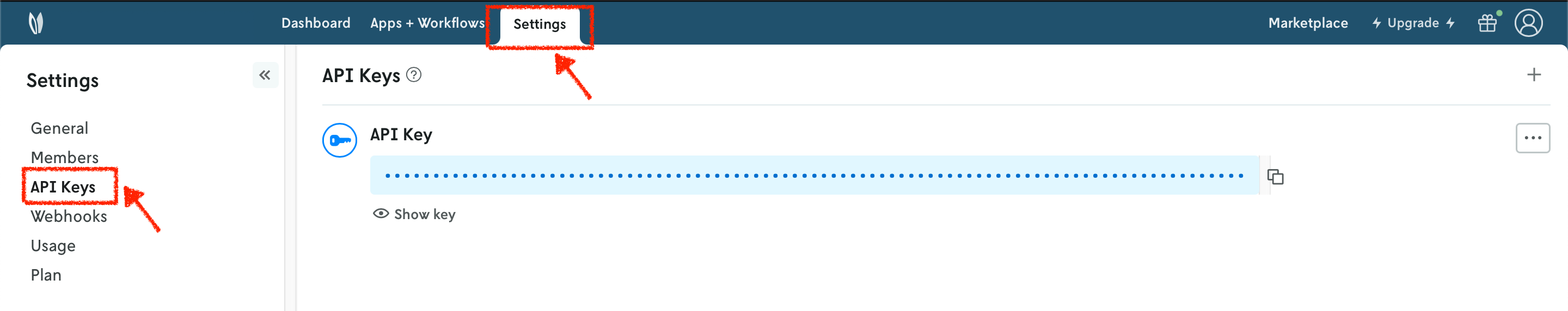
When you have your API key, it is convenient to save it as an environment variable so that you can use it for the rest of this tutorial.
6. Subscribe to a Nextmv Plan
If you already have an active Nextmv Plan, you can skip this step.
If a Nextmv member provides different instructions for activating a Nextmv Plan, please follow those instructions instead.
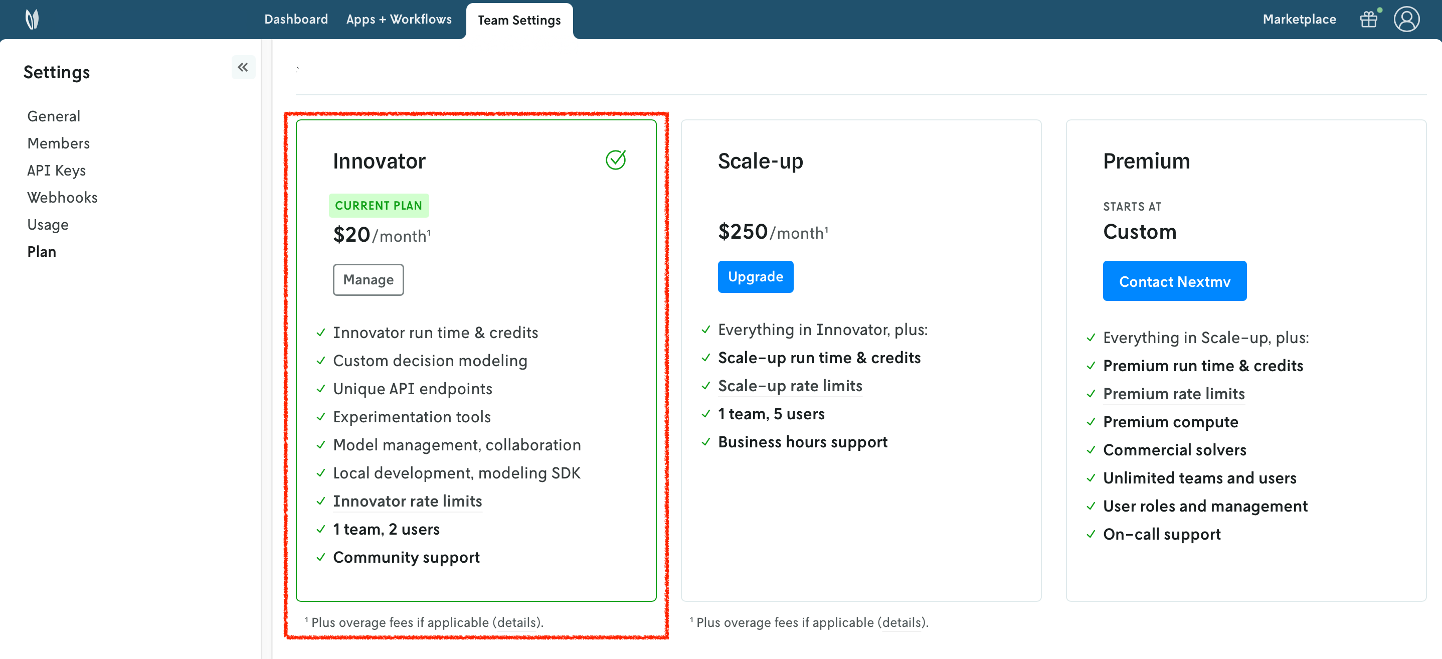
Running a custom application remotely in Nextmv Cloud requires a paid plan. However, plans come with a 14-day free trial that can be canceled at any time. You can upgrade your account and subscribe to a plan in Nextmv Console by clicking the Upgrade button in the header, or navigating to the Settings → Plan section. Upgrading to a plan will allow you to complete the rest of the tutorial.
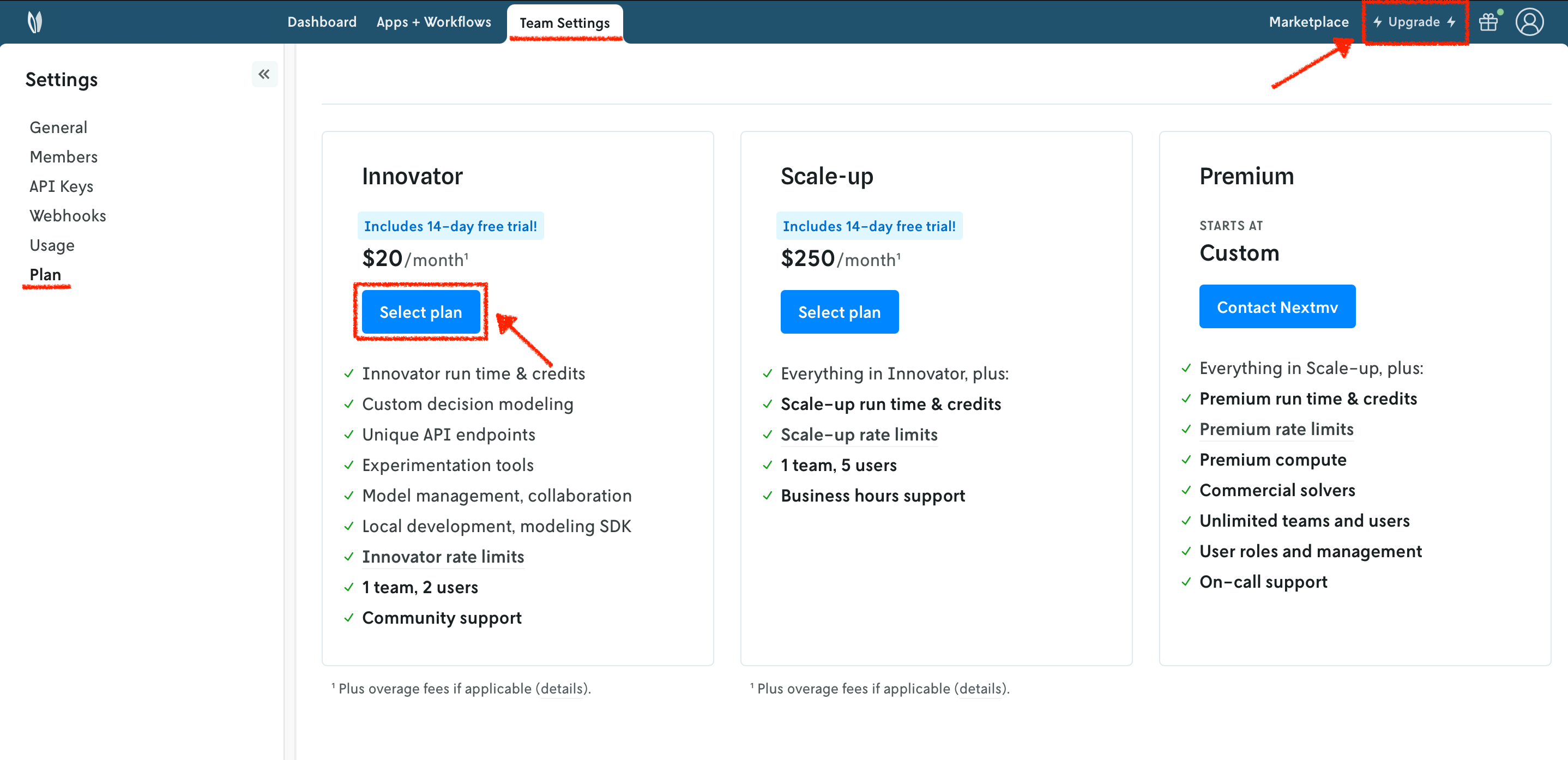
In the example shown below, you will be subscribing to an Innovator plan. A pop-up window will appear, and you will need to fill in your payment details.
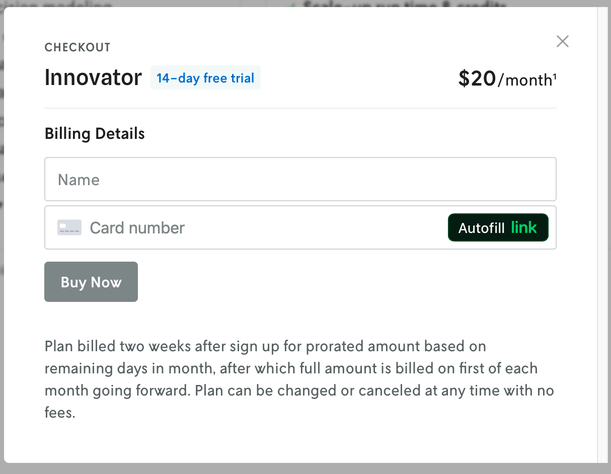
Once your account has been upgraded, you will see an active plan in your account.
7. Install the Nextmv CLI
Install the Nextmv CLI. Python >=3.10 is required. Install using the Python package manager of your choice. The CLI is available for macOS, Linux, and Windows.
After installing, configure Nextmv CLI with your account:
To check if the installation was successful, run the following command to show the help menu:
8. Create your Nextmv Cloud applications - regression, decision
To run the workflow, we need to create the two applications that are run as steps: regression, and decision.
Run the following command:
This will create a new application in Nextmv Cloud for the regression model. Note that the name and app ID can be different, but for simplicity this tutorial uses the same name and app ID. This command is saved as app1.sh in the full tutorial code. You can also create applications directly from Nextmv Console.
Now, create the application for the decision model by running the following command:
This command is saved as app2.sh in the full tutorial code.
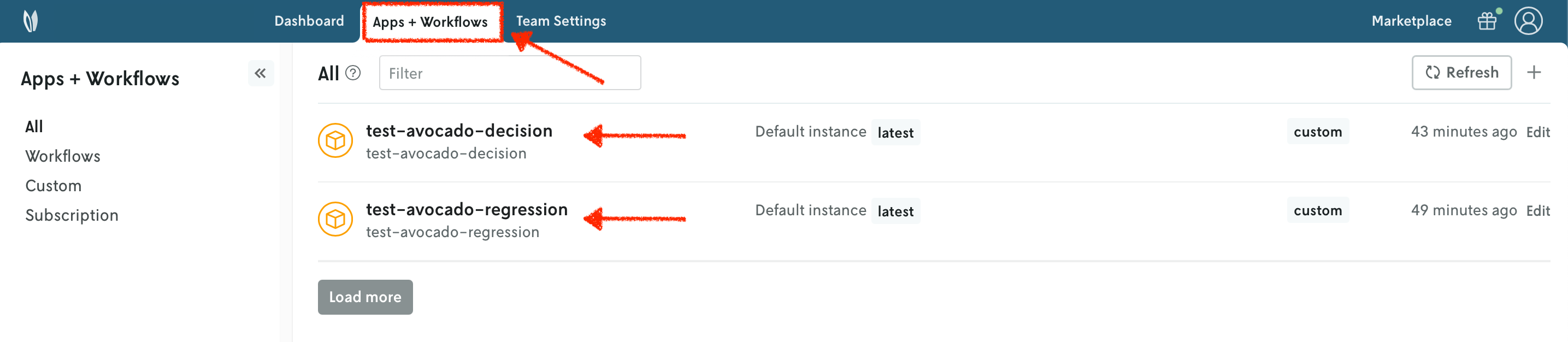
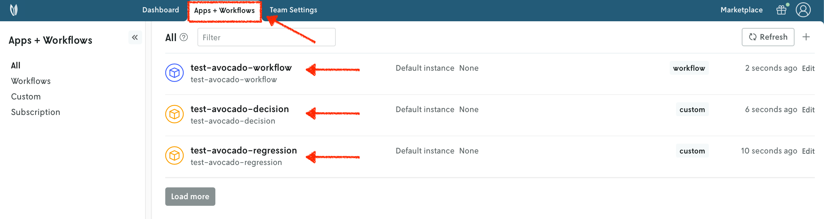
You can go to the Apps section in the Nextmv Console where you will see your applications.
9. Push your Nextmv applications - regression, decision
You are going to push your apps to Nextmv Cloud. Once an application has been pushed, you can run it remotely, perform testing, experimentation, and much more. Pushing is the equivalent of deploying an application, this is, taking the executable code and sending it to Nextmv Cloud.
cd into the regression dir, making sure you are standing in the same location as the app.yaml manifest. Deploy your regression app (push it) to Nextmv Cloud:
This command is saved as app3.sh in the full tutorial code.
Now cd into the decision dir, making sure you are standing in the same location as the app.yaml manifest. Deploy your decision app:
This command is saved as app4.sh in the full tutorial code.
You can go to the Apps section in the Nextmv Console where you will see your applications. You can click on any of the apps to see more details. Once you are in the overview of the application in the Nextmv Console, it should show the following:
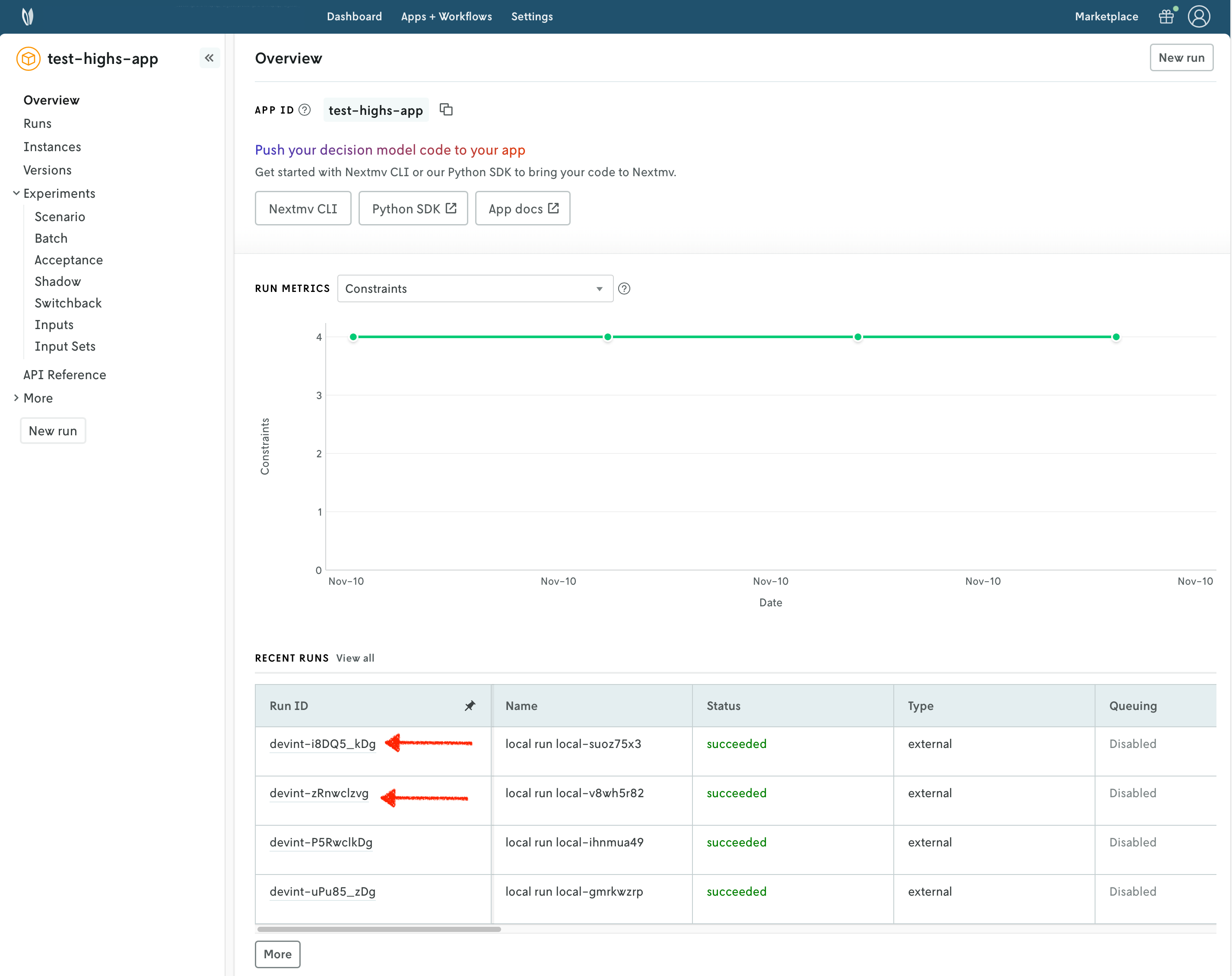
- There is now a pushed executable.
- There is an auto-created
latestinstance, assigned to the executable.
An instance is like the endpoint of the application.
10. Run the workflow application locally
Now that the regression and decision apps are pushed to Nextmv Cloud, you can run the workflow application locally. cd into the workflow dir, making sure you are standing in the same location as the app.yaml manifest.
10.1. Install requirements
First, install the requirements for the workflow application. You can do so by running the following command:
10.2. Run the application
The workflow application works with the json content format. This means that it reads json via stdin and it should write valid json to stdout. Run the app by executing the following command:
Notice that in the application logs, a URL to a mermaid diagram is provided. You can click on it to visualize the workflow executed.
After verifying that the application runs locally, we will push it and run it remotely.
11. Create your Nextmv application - workflow
Create the application for the workflow by running the following command. Notice that we are specifying that this is a workflow by using the --flow flag.
This command is saved as app5.sh in the full tutorial code.
Refreshing the overview of the applications, you should now observe the workflow app listed alongside the other two applications. Notice that this app is a different type.
12. Push your Nextmv application - workflow
To finalize deployment, push the workflow app to Nextmv Cloud. cd into the workflow dir, making sure you are standing in the same location as the app.yaml manifest. Deploy your workflow app:
This command is saved as app6.sh in the full tutorial code.
13. Run the Nextmv application remotely
To run the Nextmv application remotely, you have several options. For this tutorial, we will be using the Nextmv Console and CLI.
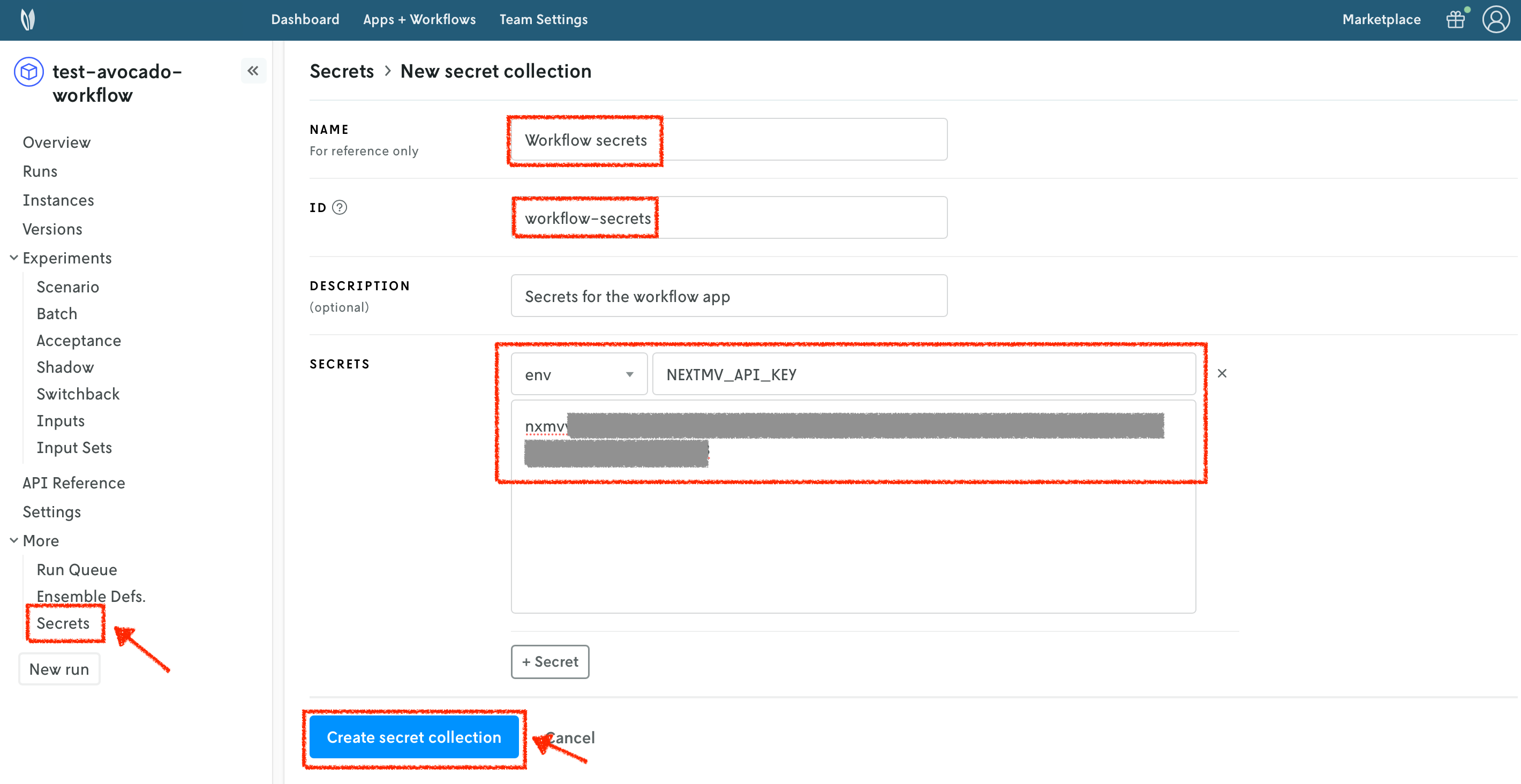
If you pay attention to the main.py of the workflow app, to run the nested Nextmv apps you use a client that needs the NEXTMV_API_KEY environment variable. Nextmv Cloud does not perform delegation, so each application is run entirely independent. To run the workflow app remotely, you must set up the NEXTMV_API_KEY environment variable as a secret.
To create a secrets collection, follow these steps:
- Select the
Secretssection of yourworkflowapplication. - Press the
+button to create a new secrets collection. - Specify a name for your secrets collection.
- Assign an ID to your secrets collection.
- You can optionally provide a description.
- Add a new
envsecret type. TheSecret locationis the name of the environment variable. TheSecret valueis the value of the environment variable. - Create the secrets collection.
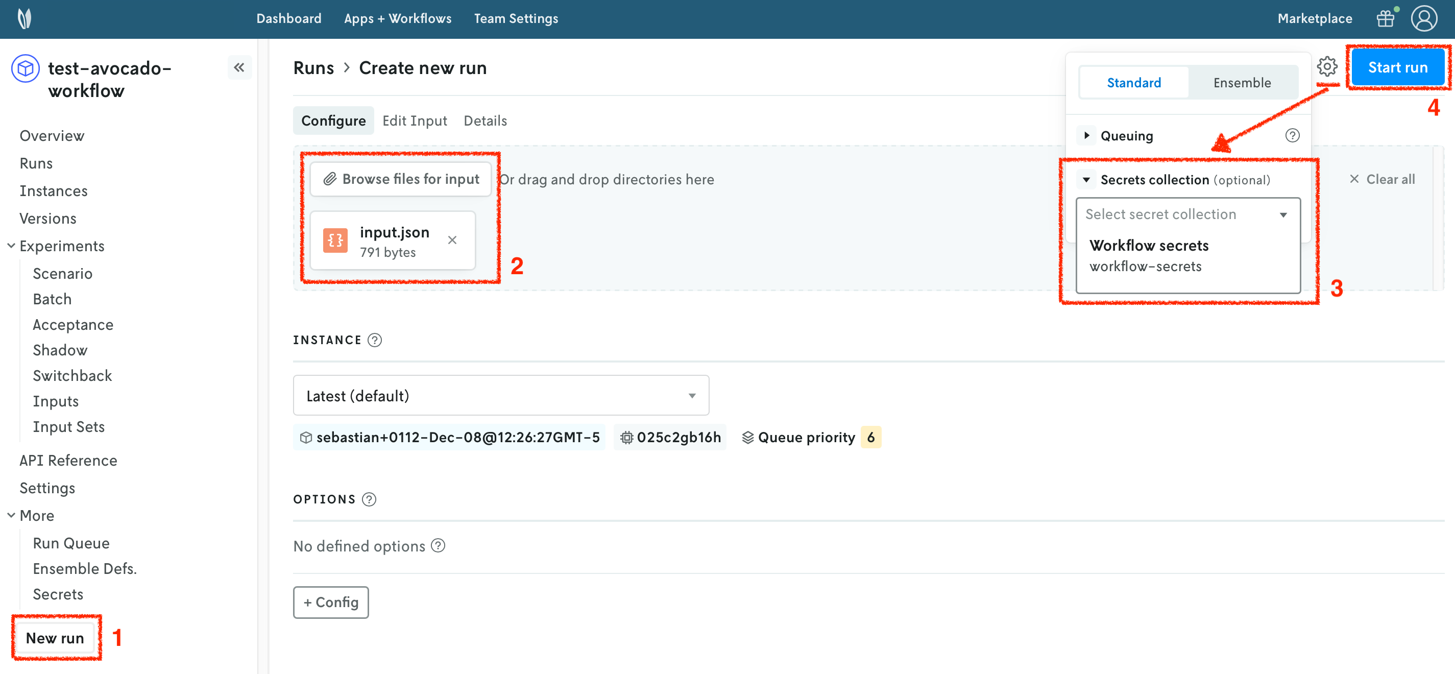
In the Nextmv Console, in the app overview page:
- Press the
New runbutton. - Drop the data files that you want to use. You will get a preview of the data. The file you need is the
inputs.jsonfile from theworkflowapplication. - Configure the run settings. Select the secrets collection you created in the previous step.
- Start the run.
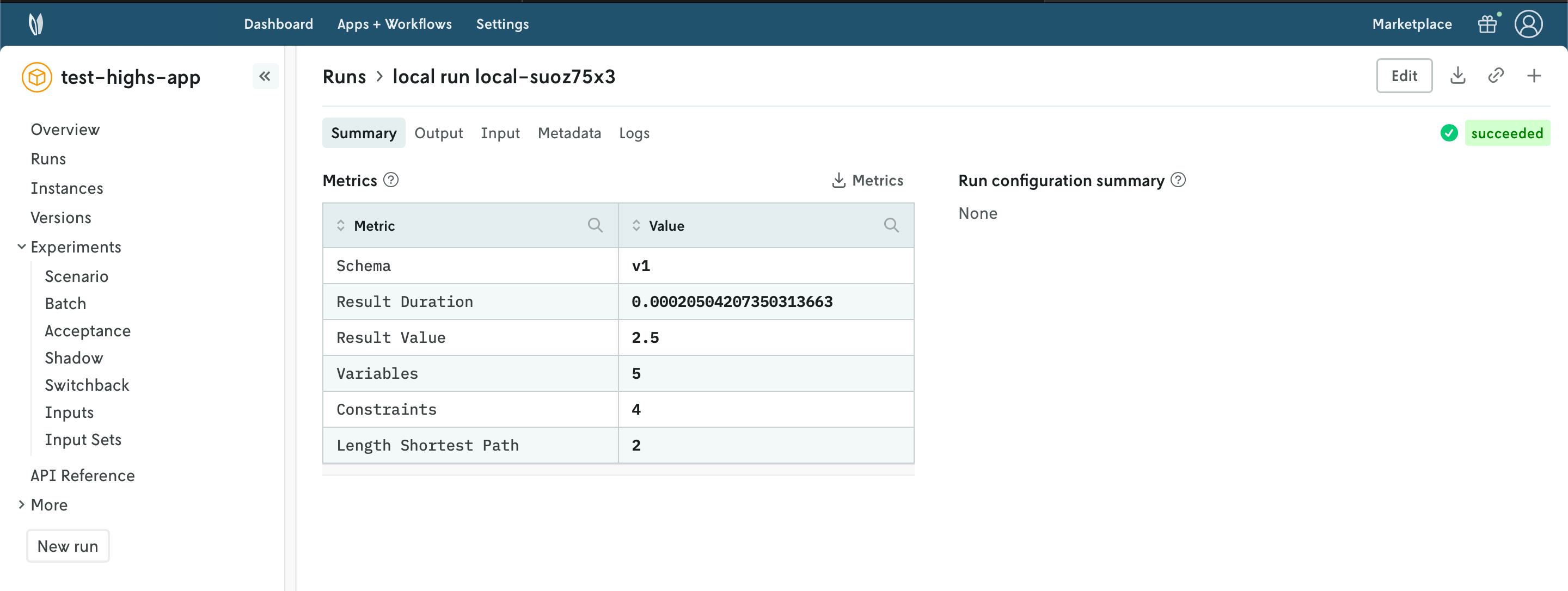
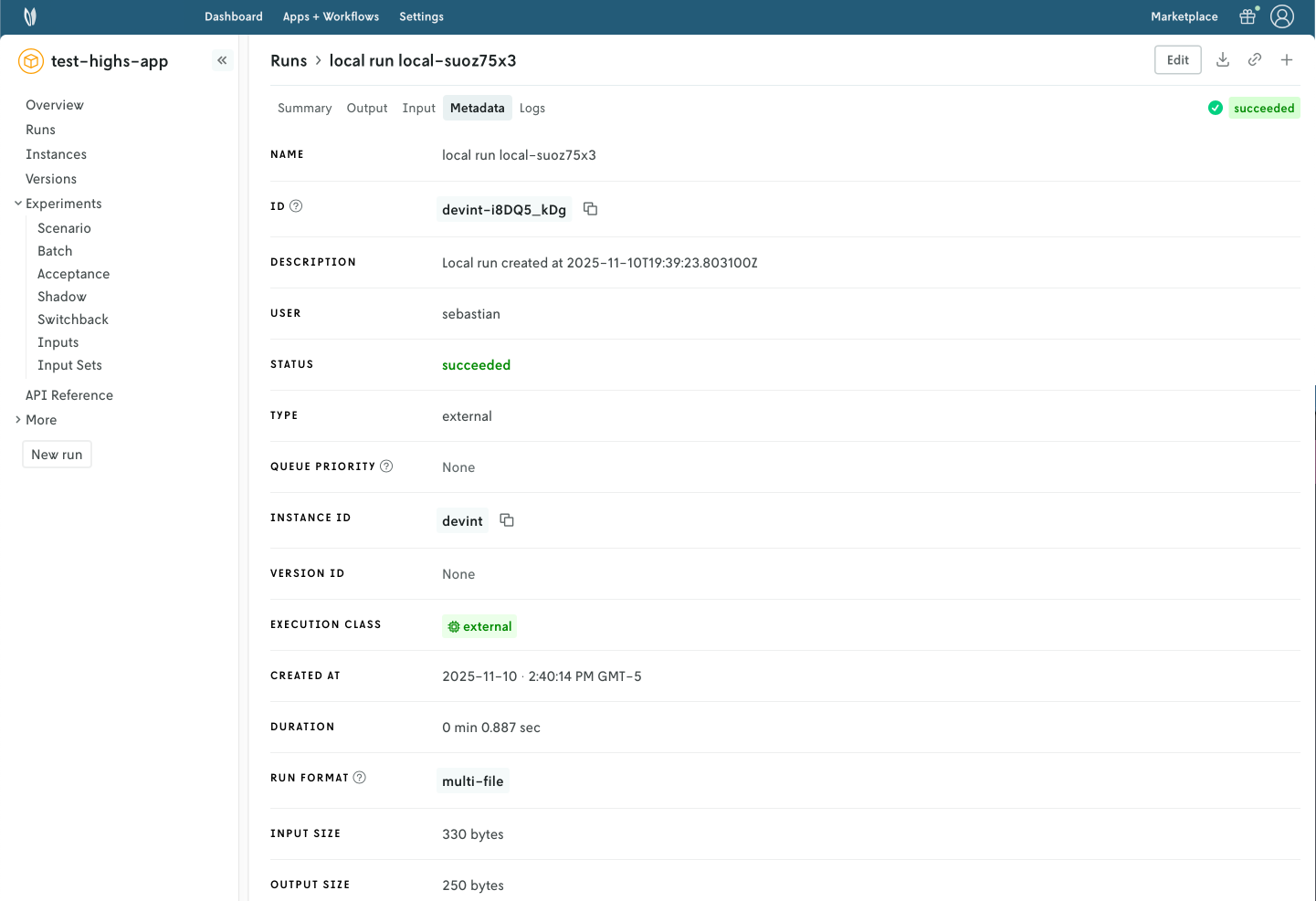
You can use the Nextmv Console to browse the information of the run:
- Summary
- Output
- Input
- Metadata
- Logs
Nextmv is built for collaboration, so you can invite team members to your account and share run URLs.
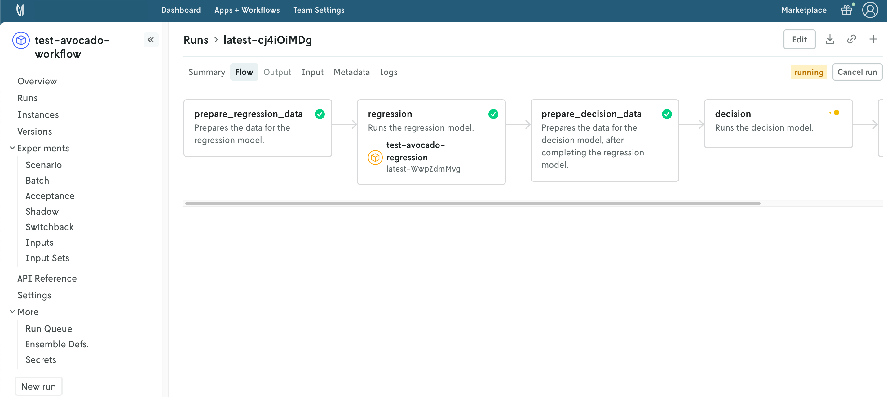
Workflow applications are special because they provide the Flow tab, where you can visualize the actual progress of the workflow and its steps.
Alternatively, you can run your Nextmv application using the Nextmv CLI. Here is an example command you can run from the root of the app.
This command is saved as app7.sh in the full tutorial code.
🎉🎉🎉 Congratulations, you have finished this tutorial!
Full tutorial code
You can find the consolidated code examples used in this tutorial in the tutorials GitHub repository. The orchestrate-multiple-models dir contains all the code that was shown in this tutorial.
For the example, you will find two directories:
original: the original example without any modifications.nextmv-ified: the example converted into the three Nextmv applications.
Go into each directory for instructions about running the decision model.