Solve a vehicle routing problem (VRP) using R and Nextmv Cloud

In this blog post, we will use Nextmv Cloud, R, and some tidyverse packages to formulate, solve and visualize a simple capacitated vehicle routing problem (CVRP). We’ll work through a sourcing scenario (meaning we’re focused on pickups rather than dropoffs) using 2 vehicles and 4 stops. 

It’s also worth noting that our cloud API supports more types of problems, including VRP with pickup and delivery, route limits, time windows, and beyond.

The primary goal of this post is to help folks who want to solve a VRP using R to get started with Nextmv more easily.

The blog post uses the new pipe operator first introduced in R 4.1, but you can of course also use magrittr’s pipe operator if you use an older version of R. In addition we make use of the following R packages:

• askpass to securely ask for an API-key,
• httr for HTTP calls,
• purrr, tidyr, and dplyr for easier data processing,
• and ggplot2 for visualization.

Let's get started.

A (brief) intro to Nextmv Cloud

Nextmv Cloud is a JSON-in-JSON-out API for automating decisions, such as how best to assign stops to vehicles. You can create a free Nextmv Cloud account (no credit card required) to follow along with the tutorial in this post. 

There are essentially three steps involved when calling our cloud API:

1. Submit a problem encoded as JSON and receive a ^runID.
2. Wait and poll the system using the ^runID until the run is completed.
3. Download the solution file encoded as JSON and further process it.

Before we can start though, we need an API key and the URL of the endpoint which you can find in the Nextmv Cloud console. After you have logged in to the console, go to the Account Page and copy your API key. Keep it safe, as it alone provides unfettered access to the cloud API.

API_KEY <- askpass::askpass("Please enter the API-Key")
URL <- "https://api.cloud.nextmv.io/v0/run"

The code above uses the askpass package to ask for API-key in a secure way. Another option is to use an environment variable and access it using ^Sys.getenv. In general we advise not to store keys directly in code files.

But before we dive into the three-step process, we first need to get our CVRP into R. 

Formulate a CVRP in R

Let’s formulate the problem first directly in R using nested lists and then go over the details. The structure corresponds to the required input schema, such that it can be converted to JSON automatically.

problem <- list(
  options = list(
    solver = list(
      limits = list(duration = "5s")
    )
  ),
  defaults = list(
    vehicles = list(
      speed = 10,
      start = list(lon = -96.659222, lat = 33.122746),
      end = list(lon = -96.659222, lat = 33.122746),
      shift_start = "2021-10-17T09:00:00-06:00"
    )
  ),
  vehicles = list(
    list(
      id = "Vehicle 1",
      capacity = 2
    ),
    list(
      id = "Vehicle 2",
      capacity = 3
    )
  ),
  stops = list(
    list(
      id = "Stop A",
      position = list(lon = -96.75038245222623, lat = 33.20580830033956),
      quantity = -1
    ),
    list(
      id = "Stop B",
      position = list(lon = -96.54613745932127, lat = 33.2259142720506),
      quantity = -1
    ),
    list(
      id = "Stop C",
      position = list(lon = -96.61059803136642, lat = 33.23528740544529),
      quantity = -1
    ),
    list(
      id = "Stop D",
      position = list(lon = -96.79586982112724, lat = 33.10492159118987),
      quantity = -1
    )
  )
)

Even without having read the full API input schema specification it is already clear what the problem is about. We have 2 vehicles with different capacities and 4 stops, each consuming one quantity. Thus we will need both vehicles to serve all stops. Each stop has a position and we use the global default settings to set a common start/end location for the vehicles as well as a speed in m/s and the date time when the shift of the vehicle starts. 

Note that instead of setting the same quantity for each stop, we could have also used the global default settings for stops. We also set an explicit time limit of 5 seconds for the solver in the options part of the problem definition. This means that the solver will stop searching for the better routes after 5 seconds. Our solver is optimized to deliver good solutions fast, but it is always a tradeoff between solution quality and runtime limits.

In the next section we use jsonlite through the httr package to convert the problem from above into the correct JSON format.

A full overview about the cloud format can be found in our docs.

Step 1: Submit the problem

First we need to submit the problem from above to our run endpoint. We can use the httr package for this purpose which can automatically convert named R lists to a JSON string. The following code constructs the correct HTTP POST request.

library(httr)
headers <- add_headers(
  Authorization = paste("Bearer", API_KEY)
)
response <- POST(
  url = URL,
  body = problem,
  encode = "json",
  headers,
  content_type_json(),
  accept_json()
)
response

## Response [https://api.cloud.nextmv.io/v0/run]
##   Date: 2022-04-26 11:02
##   Status: 202
##   Content-Type: application/json
##   Size: 49 B
## {"runID":"RUN_ID_IS_HERE"}

If successful, the returned result is a ^runID. This ID identifies your run and lets you query the status and retrieve the result.

run_id <- content(response)$runID

We assume here that the call never fails. In a production system, you would need to check that the server responded with status 202 Accepted before continuing. In addition you may want to use jsonlite directly to construct the JSON string first, before passing it to httr to have more control about the conversion process and to increase testability of your code.

Step 2: Wait until the problem is solved

The Nextmv Cloud API is designed to be regularly polled until the status of a run is final. We use purrr’s insistently function to retry the status query multiple times. Wrapping everything with possibly then ensures that we always retrieve the status as a character.

library(purrr)
query_for_status <- function(run_id) {
  response <- GET(
    url = paste0(URL, "/", run_id, "/status"),
    headers,
    content_type_json(),
    accept_json()
  )
  if (status_code(response) != 200) {
    stop("Call to API failed")
  }
  result <- content(response)
  status <- result$status
  if (!(status %in% c("succeeded", "timed_out", "failed"))) {
    stop("Run is not final yet")
  }
  status
}

robust_query_for_status <- insistently(
  query_for_status, 
  # try 5 times and wait 2 seconds between calls
  rate_backoff(pause_min = 2, pause_cap = 2, jitter = FALSE, max_times = 5),
) |> possibly(otherwise = "failed")

# We wait for at least 6 seconds before our first call as we gave the solver
# a time limit of 5 seconds.
Sys.sleep(6) 

# The following call only returns "succeeded" or "failed" if anything goes
# wrong.
robust_query_for_status(run_id)

## [1] "succeeded"

Alternatively you can write a simple for loop retrying the HTTP call until the status changes from started or requested to succeeded, failed or timed_out. Our code snippets in Go and Python give a good template for that approach.

Step 3: Download the solution

Now since we know the status is succeeded, we can download the result. Again, we use the httr package to send the HTTP GET request and also convert the response into a named list.

response <- GET(
  url = paste0(URL, "/", run_id, "/result"),
  headers,
  content_type_json(),
  accept_json()
)
solution <- content(response)

The solution variable is a list with four named elements:

• ^hop - information about our internal solver version.
• ^options - the solver options used for this run.
• ^state - the final state (aka. solution) found by the solver.
• ^statistics - some statistics about the run.

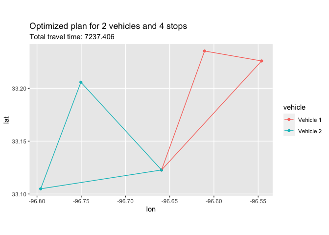
Plot the result

As a final step we show how to extract the routes from the solution and plot it.

First let’s extract the overall travel time, which is the quantity that is minimized by default.

total_travel_time <- solution$state$value_summary$total_travel_time

Then we build a data frame of all routes:

library(dplyr)
routes <- solution$state$vehicles |>
  # Collect the route for each vehicle
  map(~ tibble(vehicle = .x$id, route = list(bind_rows(.x$route)))) |>
  # Combine everything into one data frame
  bind_rows() |>
  # Unnest the list column so we get a flat table
  tidyr::unnest(route)

## # A tibble: 8 × 7
##   vehicle   id                lon   lat distance eta                       ets  
##   <chr>     <chr>           <dbl> <dbl>    <dbl> <chr>                     <chr>
## 1 Vehicle 1 Vehicle 1-start -96.7  33.1       0  2021-10-17T09:00:00-06:00 2021…
## 2 Vehicle 1 Stop B          -96.5  33.2   15568. 2021-10-17T09:25:56-06:00 2021…
## 3 Vehicle 1 Stop C          -96.6  33.2   21654. 2021-10-17T09:36:05-06:00 2021…
## 4 Vehicle 1 Vehicle 1-end   -96.7  33.1   34961. 2021-10-17T09:58:16-06:00 2021…
## 5 Vehicle 2 Vehicle 2-start -96.7  33.1       0  2021-10-17T09:00:00-06:00 2021…
## 6 Vehicle 2 Stop A          -96.8  33.2   12542. 2021-10-17T09:20:54-06:00 2021…
## 7 Vehicle 2 Stop D          -96.8  33.1   24533. 2021-10-17T09:40:53-06:00 2021…
## 8 Vehicle 2 Vehicle 2-end   -96.7  33.1   37413. 2021-10-17T10:02:21-06:00 2021…

Having everything in a data frame now lets us easily use ggplot2 to create a very basic plot of the routes as an illustrative example.

library(ggplot2)
ggplot(routes) +
  aes(x = lon, y = lat, color = vehicle, group = vehicle) +
  geom_point() +
  geom_path() +
  coord_map() +
  ggtitle(
    "Optimized plan for 2 vehicles and 4 stops",
    paste("Total travel time:", total_travel_time)
  )

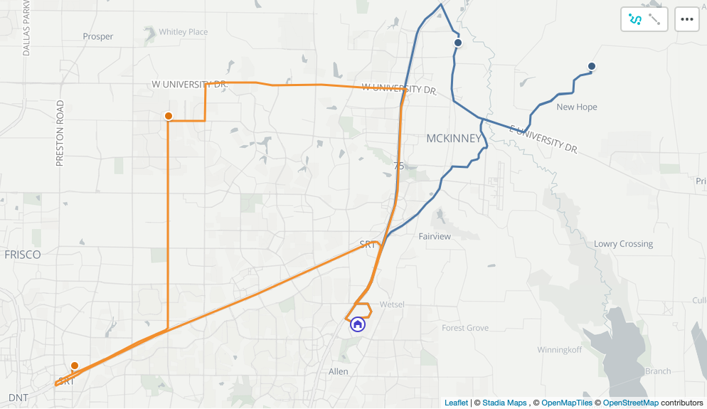
Nextmv Cloud also offers interactive visualizations out of the box that utilize the real road network:

How to continue from here

Congratulations, you’ve successfully solved a simple CVRP with R and the Nextmv Cloud API. There’s more to explore from here. 

For example, if you want to integrate the Nextmv solver into a Shiny application, take a look into promises to better build a responsive app using asynchronous calls to our API. And if you are interested in the broader spectrum of optimization packages in R, you should definitely take a look at CRAN’s Task View on Optimization and Mathematical Programming.

There are also several other demo input files to explore within the Nextmv Cloud console. It’s also easy to experiment with many other features such as compatibility attributes, penalties, backlogs, route limits, vehicle initialization costs, and more. 

It’s easy to create a free Nextmv Cloud account (no credit card required). We have options for more customization. If you want to talk to the Nextmv team, just contact us.

‍

Editor's note (November 17, 2022): This post was updated to reflect the current API key location in console.