


Efficient scheduling is critical across industries and companies of all sizes – from education and healthcare to retail and beyond. Here are just a few examples of scheduling questions:
Routing: How do I effectively schedule my fleet of drivers for different times of day with varying orders?
Staffing: How do I schedule workers for simultaneous events requiring different skills and shift lengths?
Cloud computing: How do I effectively allocate resources like compute and memory across a cloud platform to meet user demand?
Scheduling in the context of decision automation
Scheduling is the process of assigning resources to a task, unit of time, or space. When it comes to workforce scheduling, there are many factors that are often taken into consideration including business requirements like shift minimums and maximums, skill sets, demand, and cost. And in many cases, those variables may shift depending on seasons, day of the week, or time of the day.
Like routing, scheduling is a type of decision-making. There are usually people (or teams) dedicated to solving this problem for an organization. Sometimes it’s done manually using spreadsheets or a simple interface in a process that can be tough to scale. Decision automation uses algorithms to find optimized scheduling solutions that look to cover demand, reduce surplus, and mirror business logic like shift lengths and worker skill sets. Automating scheduling decisions frees these teams up from repeated manual tasks,allows them to manage larger operations, and supports them in taking on more strategic roles.
Route and schedule optimization
At Nextmv, we often start helping customers by finding solutions to their routing problems. When optimized routes are returned, they may realize that they need to rethink the number of drivers they are scheduling to properly meet demand. Here’s where the decision automation platform comes into play.
In this post, we’ll solve a workforce scheduling problem that stems from a relatively simple vehicle routing problem (VRP). We’ll tackle this problem in two parts. In Part 1, we’ll calculate order demand and the required number of drivers per hour. In Part 2, we’ll use that data to create a shift schedule.
Already know what your hourly driver demand looks like? Skip to Part 2!
Part 1: Calculate drivers required per hour
Before we can schedule drivers, we need to:
- Get an understanding of how many orders we typically have in a day
- Generate scenarios to represent varying order times and locations
- Calculate drivers required per hour
We’ll walk through each step of the process in detail below.
Step 1: Review historical demand
The first step in solving our workforce scheduling problem is understanding demand. In this case, we’ll think about demand in terms of delivery orders in a specific region over the course of one day.
We’ll use historical data consisting of:
- Number of orders per hour and their locations
- Location of distribution center
- Service region around the distribution center
Here’s an example of order volume for each hour of the day, starting at midnight:
[3,1,4,5,12,13,14,12,14,15,15,16,20,21,24,26,20,21,14,11,9,4,4,3]
In our example we’ll say we have 301 orders coming in during the course of the day that we’re analyzing.
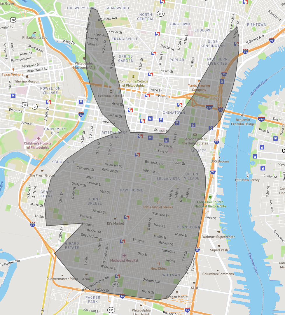
The delivery center for our example is located at: -74.9848, 40.10626. Here’s a mockup of a busy (some may say hoppin’!) service region:
Step 2: Create multiple scenarios to account for order time and location variation
At this point, we have everything we need to begin understanding what demand looks like. However, we don’t want to plan based on only one scenario since it's highly unlikely that we’ll see the exact same number of orders each hour from the same locations.
To make sure we’re prepared for the demand that might occur, we’ll create 10 scenarios that randomize when and where orders are placed in the service region. In our case, we’ll randomize orders within 60-minute windows. If you are observing order distribution at a higher resolution, you can easily match it with blocks of 10 minutes and so on. The same can be done for location so as to randomize order location within specific neighborhoods rather than across the entire service region. Creating these randomized scenarios based on historical data keeps the total order volume constant while giving us a good idea of variation in order placement so we can plan effectively.
Next, we’ll account for business logic (or constraints) surrounding the delivery process. The following constraints will remain a constant for each scenario.
- Delivery time: The duration of the hard time window of when an order should be delivered (in seconds)
- Target seconds: The ideal duration between when the order is populated in the system and the time that the delivery is made (in seconds)
- Lateness penalty: Value penalty for arriving late
- Pickup duration: How long the pickup will take (in seconds)
- Dropoff duration: How long the dropoff will take (in seconds)
- Max batching: How many orders can be batched together in a single route
- Measure type: How routes are calculated (e.g., Haversine or real-road networks)
Then we’ll run the orders and constraints through a custom script that randomizes order times and locations within the given delivery area and writes the result to a file following the Nextmv Cloud input schema. The program produces one input file for each generated scenario – so in our case, 10 files.
Here’s a (truncated) example of one of the Nextmv Cloud input files created by the script:
Step 3: Generate vehicle routes for each scenario
To start planning the schedule, we need to get a better sense of what optimized routes and driver requirements look like for each of these scenarios. The files we just created above will help us do this.
Let’s use Nextmv Cloud. Once we’ve logged in, we can drop one of our newly generated input files directly into the demo space, click “run,” and see the optimized routes on the map. To run all 10 scenarios in parallel and speed up the process, we will use the Nextmv Cloud API.
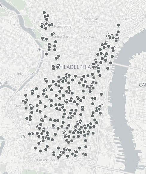
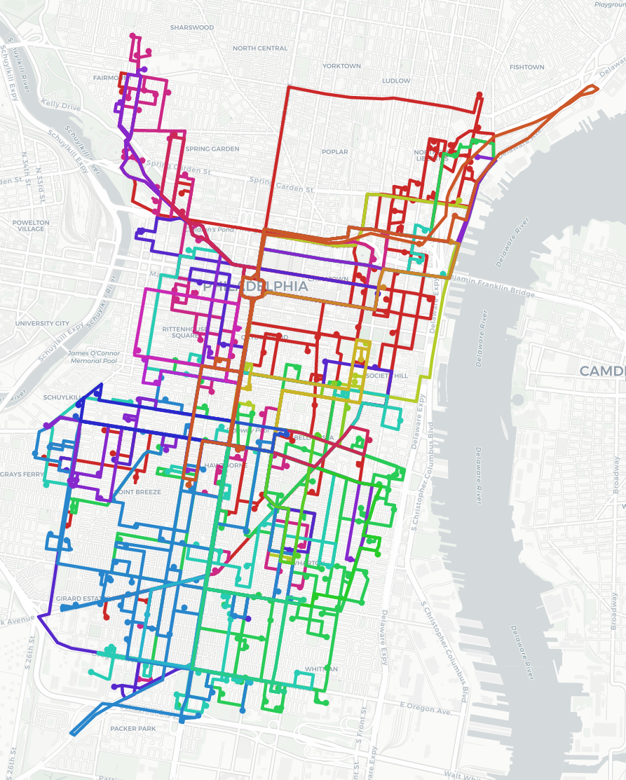
Below are examples of what the stops and optimized routes for one scenario (or input file) look like on the map.
The Nextmv Cloud JSON output details the optimized solution per scenario following this schema. We’ll focus closely on how many vehicles are being used in each scenario.
Here’s a truncated version of an output file that shows a vehicle and a few of it stops along with details like estimated time of arrival (ets) and estimated time of service (ets).
Step 4: Calculate number of drivers required per hour per scenario
The Nextmv Cloud output for each delivery scenario identifies the number of vehicles (and therefore drivers) required, in addition to the times they’re actively engaged, as denoted by their routes. This gives us an idea of the drivers required to effectively handle the order demand.
Scheduling generally happens in shifts so we’ll want to identify drivers needed per hour. We’ll break the day into 24 time slots for each hour of the day to better understand the hourly driver demand per scenario. We’ll end up with 10 arrays of 24 integers representing the demand per hour.
Step 5: Create a single array of driver demand per hour
Now that we know how many drivers we need per hour per scenario, we’ll want to merge the results from all the scenarios to answer the question: How many drivers are required per hour to handle order demand across our scenarios?
There are many different ways to merge the results from these scenarios. Here are two we explored:
- Take the maximum for each hour. This is a conservative approach that will likely cover all demand but may also result in scheduling too many shifts (where workers are not active).
- Take an average for each hour. This approach is less conservative with fewer unutilized shifts but may not always cover demand.
We decided to go with option 2 to reduce the surplus. After merging with this method, we got the following array:
[4, 4, 3, 3, 2, 3, 2, 2, 3, 4, 6, 7, 6, 5, 7, 7, 5, 7, 7, 8, 8, 7, 8, 6]
So at 12:00 AM local time, 4 drivers are required to meet average delivery demand. At 4:00 AM we only need 2 drivers. And so on.
Part 2: Create a shift schedule that covers hourly driver demand
Now we’ll take the single array of numbers and do the following to create a shift schedule:
- Create an input file
- Solve the scheduling problem
- Analyze the solution
Step 1: Create an input file for scheduling engine
We’re almost there! We have a solid idea of order demand and the amount of drivers we’ll need to cover that demand. Next, because this is a scheduling problem, we’ll want to think about drivers in terms of worker shifts.
In this case, we also need to represent the following shift constraints:
- shift_length_min (no shorter than two hours)
- shift_length_max (no longer than 8 hours)
Here’s what the input looks like for our scheduling engine:
Step 2: Solve the scheduling problem
We’ll use the Nextmv scheduling engine to transform the hourly drivers needed into shifts. Our scheduling engine will seek to cover all demand with as little surplus (or unutilized workers) in as few shifts as possible while adhering to all constraints.
Here’s what an example output file looks like:
Step 3: Analyze the results
If we take the JSON output and plot it, here’s what it looks like in terms of demand and surplus.
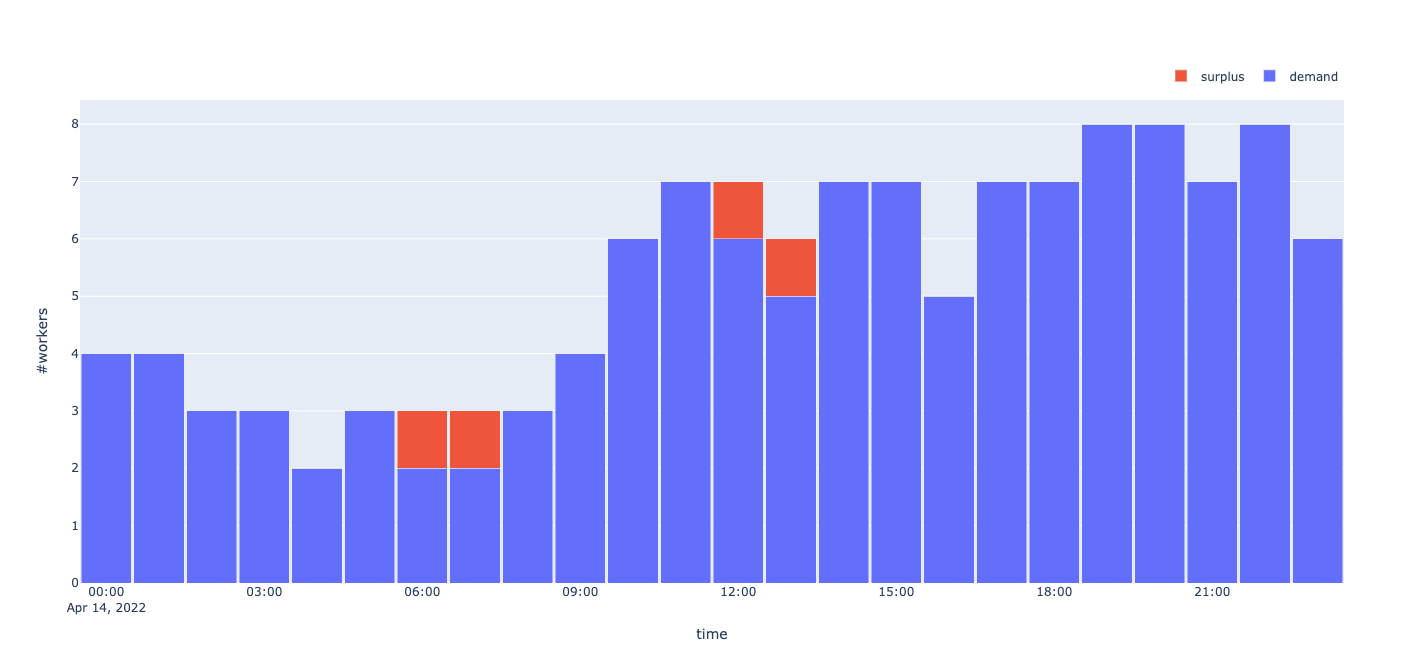
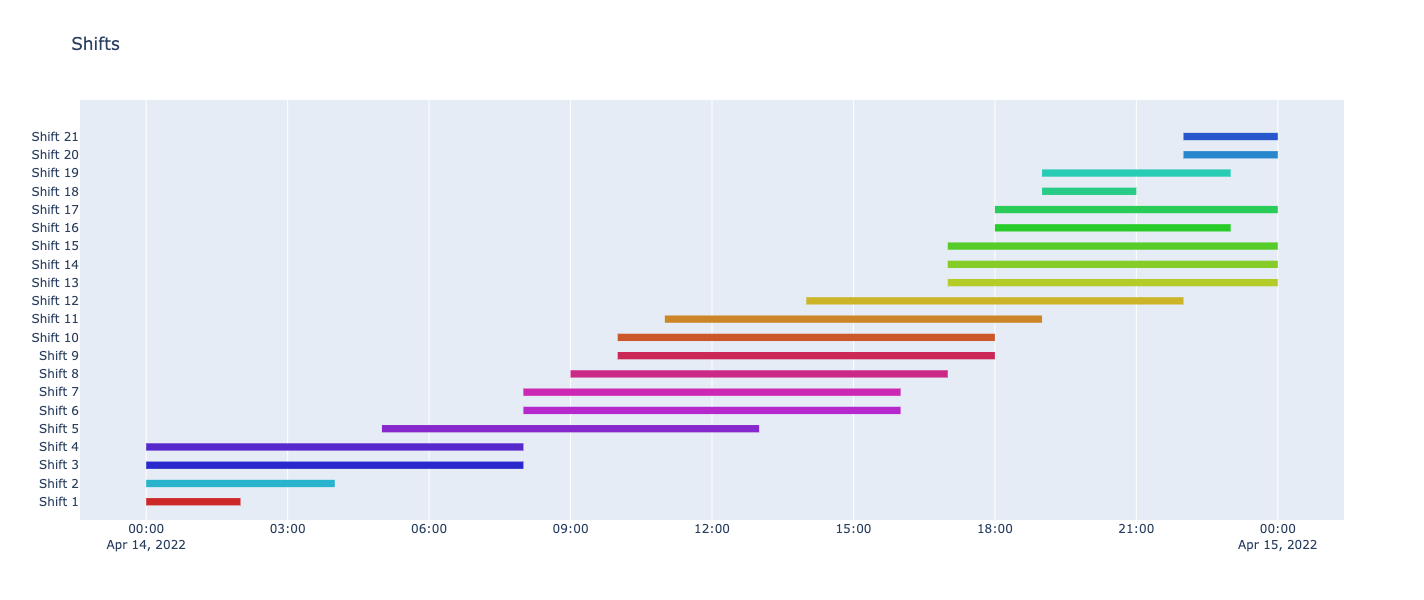
We have covered a demand of 124 worker hours by scheduling 21 worker shifts. This resulted in a 4-hour surplus over the course of the day when workers are scheduled but not active.
And here are each of the 21 shifts plotted by time. All of the shifts are between 2 and 8 hours long, which aligns with our desired business logic for our scheduling problem.
Learn more about scheduling with Nextmv
Automating your workforce scheduling decisions is just one way that Nextmv’s decision automation platform can increase your team’s efficiency and help your company scale.
Ready for all of your operational decisions to look and feel the same with our decision automation platform? Get started routing with Nextmv Cloud and reach out to us to get started with scheduling.


